
Choose inventory analysis methods by the decision you need to make: ABC for consumption-value priorities, XYZ for demand variability, EOQ for order size, safety stock and reorder points for replenishment, and turnover or aging for stock exposure. This guide helps planners and analysts select a method, prepare its inputs and interpret the result.
Choose a method for your inventory decision
| Decision and method | Inputs and interpretation |
|---|---|
| Which items deserve value-based attention? ABC analysis | Usage and unit cost for one period. Rank consumption value; add criticality and supply risk before setting service policies. |
| Which items have more variable demand? XYZ analysis | Demand in equal time intervals, with explicit missing-value rules. Variability groups do not establish seasonality or forecast accuracy; zero-mean demand needs separate handling. |
| What is moving or sitting idle? FSN analysis | Movement history, recency and a stated observation window. Definitions vary: a coverage-based label is different from a transaction-based label. |
| How much should be ordered? EOQ | Annual demand, cost per order and annual holding cost per unit. Compare feasible quantities and constraints; EOQ does not set the reorder trigger. |
| When should replenishment start? Safety stock and reorder point | Demand, lead time, variability and a defined service target. Match units and review policy; assess inventory position, not only the shelf balance. |
| How much stock supports sales? Inventory turnover | COGS and average inventory at cost over the same period. Compare similar products and service outcomes; higher is not always better. |
| Which stock needs recovery review? Aging and obsolescence review | Receipt/expiry dates, remaining stock, demand and recovery assumptions. An age bucket or expected-loss model is not an accounting valuation. |
| Why do records differ from physical stock? Cycle counts and DMAIC | Count results, movement cutoffs, adjustments and reason codes. Reconcile first, then investigate recurring causes and test corrective action. |
Prepare and validate the data first
State the data grain: for example, one SKU–location balance at a specified snapshot time, with a separate movement table containing one transaction per row. Record the observation period, unit of measure, currency and cost basis. Keep legitimate multiple lots or locations; do not remove them as duplicates just because the SKU repeats.
- Reconcile opening units + receipts − issues + signed adjustments to closing units at the same scope. For example, 100 + 40 − 30 − 2 = 108 units. Explain transfers, returns and count adjustments explicitly.
- Distinguish zero demand from a missing record. Resolve duplicate transaction IDs and investigate negative stock or cost; do not silently replace suspicious values with zero.
- Check one SKU manually, then test zero demand, a missing period, a classification cutoff and a seasonal item. Compare the proposed action with service, capacity, expiry and supplier constraints.

Tools for Inventory Analysis
Start with the business question and data quality, then choose software. A dashboard cannot correct missing transactions, inconsistent units or an unsuitable inventory policy.
1. Inventory Management Software
- ERP systems: Use an integrated system when inventory needs to connect with purchasing, sales and finance. Check transaction controls, unit conversions, location-level stock, integrations and reconciliation. Timely visibility depends on accurate event capture and updates; software alone does not ensure it.
- Standalone inventory software: Compare order and stock workflows, integrations, audit trails, implementation effort and total cost. Do not select by company size alone. The former TradeGecko/standalone QuickBooks Commerce offering is not a current shortlist option: Intuit confirms its discontinuation.
2. Spreadsheet Software
- Microsoft Excel and Google Sheets: Useful for a controlled prototype, reconciliation or small repeatable analysis. Protect formulas, document units and assumptions, and separate imported data from calculations. Check duplicates and reconcile totals before using pivot tables or charts; set an owner and version-control process.
3. Business Intelligence (BI) Tools
- Business intelligence tools: Use dashboards to compare inventory, demand and service measures across products and locations. Keep stock snapshots separate from transaction facts and document refresh timing. Microsoft’s modelling guidance stresses consistent fact-table grain: a join must not multiply stock balances by the number of sales rows.
4. Barcoding and RFID Systems
- Barcodes and RFID: These capture identifiers and events; records update only when the scanning workflow and systems are connected correctly. A product barcode need not identify an individual physical unit. GS1 distinguishes product, batch/lot and serial-level identification. Choose the required level and test missed or duplicate scans.
5. Warehouse Management Systems (WMS)
- Warehouse management systems: Evaluate receiving, putaway, location control, picking, replenishment and shipping against your actual warehouse workflows. Test barcode integration, lot/expiry support, exception handling and stock reconciliation. Measure any improvement against a baseline rather than assuming a system guarantees accuracy or productivity.
Techniques for Inventory Analysis
Use the following methods together where appropriate. Segmentation sets review priorities; replenishment models set quantities or triggers; counting and traceability check physical records and movement.
1. ABC Analysis
For consumption-value ABC analysis, calculate each SKU’s annual usage × unit cost, rank descending and apply documented cumulative-value cutoffs. Use the same period and cost basis for every SKU. Classes describe value concentration, not physical quantities or item criticality:
- Class A: The highest-ranked group by cumulative consumption value under your chosen cutoff. Review frequently, while also considering supply risk and criticality.
- Class B: The next cumulative-value band. Assign review effort using both its value contribution and operational risk.
- Class C: The remaining lower-value band. Low consumption value does not mean an item is safe to run out of; a low-cost critical spare can stop production.
Teaching example: 1,000 units/year at ₹10 each contribute ₹10,000 annual consumption value; 100 units/year at ₹80 contribute ₹8,000. Rank the first item higher despite its lower unit price. Use the ABC calculator with separate cost and usage inputs, and document how items crossing a cutoff are assigned.
2. Economic Order Quantity (EOQ)
For the basic EOQ model, Q = √(2DS/H), where D is units/year, S is cost/order and H is holding cost/unit/year. Assume stable, known demand, fixed ordering and holding costs, receipt of the lot together and no shortages. EOQ balances ordering and cycle-stock holding costs; it is not a universal purchasing optimum.
3. Just-In-Time (JIT) Inventory
Just-in-time is an operating approach, not a stock-analysis formula. Toyota’s account of JIT describes producing required parts in required quantities. Reliable replenishment, quality and process coordination matter. Cutting buffers without addressing disruption exposure can worsen service.
4. Safety Stock Analysis
Safety stock reduces shortage risk under an explicit demand and supply model; it cannot guarantee availability through every disruption. With fixed lead time L and independent, identically distributed daily demand, SS = z × σd × √L. Here σd is the standard deviation of daily demand in units, L is days, and z is a dimensionless normal quantile for the target cycle-service level (probability of no stockout in a replenishment cycle), not fill rate.
5. Demand Forecasting
Forecast future demand at the product, location and time level used for replenishment. Recorded sales can understate demand during stockouts. Compare methods on later periods excluded from training, at the required horizon; review both error and bias. Forecasting: Principles and Practice explains why fitted accuracy is not forecast accuracy and why MAPE fails with zero actuals.
6. Inventory Turnover Ratio
Inventory turnover = cost of goods sold during the period ÷ average inventory at cost for that period. Use a positive denominator and matching currency, scope and valuation basis. For annual COGS ₹900,000 and opening/closing inventory ₹100,000/₹80,000, the two-point average is ₹90,000 and turnover is 10 turns/year. More frequent balances better represent seasonal stock. High turnover may also accompany shortages; assess it alongside service.
7. Lot Tracking and Traceability
Link product and lot/serial identifiers to receipts, movements, transformations and shipments so affected stock can be located. Test a mock trace in both directions and reconcile quantities; retaining a lot-number column alone is not complete traceability. GS1’s traceability standard provides the identification and event-recording framework. Sector-specific legal requirements need separate review.
8. Reorder Point Formula
For continuous review, reorder point ROP = expected demand during lead time + safety stock. With mean demand d units/day and fixed lead time L days, expected lead-time demand is d × L. Compare the trigger with inventory position: on-hand + on-order − outstanding demand commitments, counted once. Avoid subtracting allocations twice if they are already reflected in available stock. A periodic-review policy also needs to cover its review interval.
9. Cycle Counting
Cycle counting checks selected items and locations on a rolling schedule. Prioritize by discrepancy history, value, movement and criticality. Control transaction cutoffs or track movements during the count; investigate variances before approved adjustments. Track repeat causes and recounts rather than treating a corrected system balance as proof the process is fixed.
10. Six Sigma
Use DMAIC: Define, Measure, Analyze, Improve, Control for a recurring inventory-process problem. For pick errors, define the defect and denominator, validate the measurement, investigate causes, pilot a change and monitor recurrence. A before/after improvement alone does not establish causation.
11. Pareto Analysis
A Pareto chart ranks categories by a chosen measure such as discrepancy cost or count. Measure the actual concentration; 80/20 is not a required split. ABC applies a related ranking idea to inventory items. A Pareto chart highlights priorities but does not prove root causes.
12. Inventory Aging Reports
Define age from a stated event, such as original receipt or manufacture, and use non-overlapping buckets (for example, 0–30, 31–60 and 61–90 days). Internal transfers should not silently reset economic age. Combine age with movement, expiry, expected demand and recoverable value; old inventory is not automatically obsolete. Review assumptions in the obsolescence calculator before using its scenario estimate.
Worked examples: separate order size from timing
Order-size example: D = 10,000 units/year, S = ₹50/order and H = ₹5/unit/year give EOQ = √(2 × 10,000 × 50 ÷ 5) = 447.21 units. If units must be whole, compare feasible nearby quantities using annual relevant cost DS/Q + HQ/2. Do not simply round up and declare it optimal. If D is zero, this model creates no demand-driven order; H must be positive. Review minimum orders, pack sizes, discounts, expiry and capacity separately.
Reorder example: independent daily demand has mean 100 units and standard deviation 20 units; fixed lead time is 4 days. With z = 1.65 (approximately 95% cycle-service level under a normal approximation), SS = 1.65 × 20 × √4 = 66 units and ROP = 100 × 4 + 66 = 466 units. If variability is zero, this model’s safety stock is zero, not a guarantee against unmodelled disruption. Keep precision during calculation; rounding a final stock threshold upward may be a chosen whole-unit policy, unlike optimizing EOQ.
These are separate teaching scenarios, not observed business results or one combined policy. The safety-stock shortcut is unsuitable without adjustment for variable lead time, dependent demand, strong seasonality or intermittent demand. See the variable-demand and lead-time guide. The underlying EOQ and continuous-review assumptions are covered in MITx SCM Key Concepts, sections 2.3.3 and 2.3.8. The OpenStax turnover methodology supports the same-period COGS/average-inventory calculation above.
Next action: choose one decision from the table, reconcile a small sample and run the linked calculator with documented assumptions. Record the proposed action, owner and review date, then compare the outcome with both inventory cost and customer service.





2 Comments